Data Compression via Dimensionality Reduction: 3 Main Methods

(This article originally appeared on KDNuggets.com here. For more, visit https://www.kdnuggets.com/)

Lift the curse of dimensionality by mastering the application of three important techniques that will help you reduce the dimensionality of your data, even if it is not linearly separable.

Why reduce the dimensions of data?

If you are in data science for quite some time, you must have heard this phrase:

Dimensionality is a curse.

This is also referred to as the curse of dimensionality. You can learn more about this term here.

Overall, some of the common disadvantages of high dimensional data are:

1. Overfitting the model
2. Difficulties in clustering algorithms
3. Very hard to visualize
4. There might be some useless features in your data
5. Complex and costly models

There are other disadvantages too, which you can search and look for details on Google.

In this article, we are going to discuss 3 important and famous techniques, which will help you in reducing the dimensions of your data while maintaining useful features or information.

These 3 essential techniques are divided into 2 parts.

1. Linear dimensionality reduction

• PCA (Principal Component Analysis)
• LDA (Linear Discriminant Analysis)

2. Non-linear dimensionality reduction

• KPCA (Kernel Principal Component Analysis)

We will discuss the basic idea behind each technique, practical implementation in sklearn, and the results of each technique.

PCA (Principal Component Analysis)

Principal Component Analysis is one of the most famous data compression technique that is used for unsupervised data compression.

PCA helps us to identify the patterns in the dataset based on the correlation between them. Or simply, it is a technique for feature extraction that combines our input variables in such a way that we can drop the least important ones while retaining the important information in the dataset. PCA finds the direction of the maximum variance and projects the data into lower dimensions. The principal components of the new subspace can be interpreted as the direction of maximum variance given the constraint that the new feature axes are orthogonal to each other.

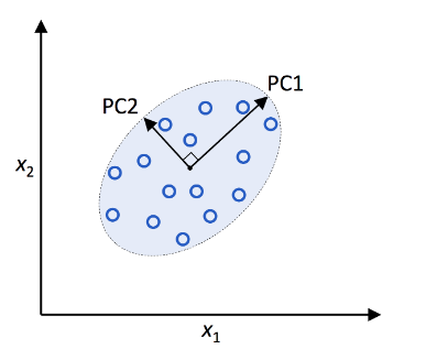
Image Credits: Python Machine Learning repo.

Here, x1 and x2 are the original feature axes, and PC1 and PC2 are the principal components.

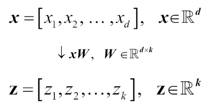
When using PCA for dimensionality reduction, we construct a transformation matrix W, which is d x k dimensions, that allows us to map a sample vector x onto a new k-dimensional feature subspace that has fewer dimensions than the original d–dimensional feature space.

Typically k is very less than d, so the first principal component has the maximum variance, and so on.

PCA is highly sensitive to data scaling, so before using PCA, we have to standardize our features and bring them on the same scale.

PCA is simple to implement from scratch in Python, and it is given as a built-in function in sklearn. To check a from scratch implementation, refer to this repo. We will review the implementation in sklearn.

Sklearn Code:

First of all, we have to import a dataset and preprocess it.

import pandas as pd
df = pd.read_csv('https://archive.ics.uci.edu/ml/'
                 'machine-learning-databases/wine/wine.data',
                  header=None)
print(df.head)

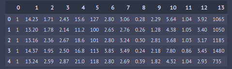
This is our dataframe with class labels (1,2,3) in 0th column and features in 1–13 columns. Let’s assign those to X and y.

X = df.iloc[:, 1:] #all rows, columns starting from 1 till end
y = df.iloc[:, 0] #all rows, only 0th column

Now let’s split the dataset into training and testing portions.

from sklearn.model_selection import train_test_split
X_train, X_test, y_train, y_test = train_test_split(X, y, stratify=y, test_size=0.2, random_state=0)

Now since we have split the dataset, let’s apply a Standard Scaler to standardize our features.

from sklearn.preprocessing import StandardScaler
sc = StandardScaler()
X_train_std = sc.fit_transform(X_train)
X_test_std = sc.transform(X_test)

Now, all we have to do is to perform PCA on it.

from sklearn.decomposition import PCA
#pca = PCA()

Now, we can pass either how much percent of variance do we want to keep or the number of components. For example, if we want to store 80% of the information on our data, we can do pca = PCA(n_components=0.8), or if we want to have 4 features in our dataset, we can do pca = PCA(n_components=4).

pca = PCA(n_components=2)
X_train_pca = pca.fit_transform(X_train_std)
print(X_train_pca.shape)

And we can see that we have jumped from 13 features to 2 features. In order to check how much information we are saving, we can do

pca.explained_variance_ratio_

For visualization purposes, we did 2 features, as 2 features can be easily visualized. And we can see that the first feature has ~36% of the information and 2nd feature has ~18% of the information. So we lost 11 features while we still have 55% of the information, which is really cool.

Let’s plot these 2 features.

colors = ['r','b','g']
markers = ['s','x','o']
for l,c,m in zip(np.unique(y_train), colors, markers):
    plt.scatter(X_train_pca[y_train==l,0],
                X_train_pca[y_train==l,1],
                c=c, label=l, marker=m)
plt.title("Compressed Data")
plt.xlabel("PC1")
plt.ylabel("PC2")
plt.legend()
plt.tight_layout()
plt.show()

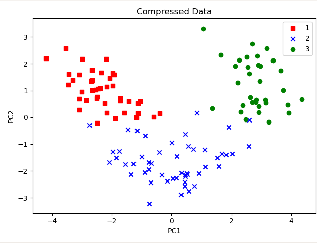
Now you can apply any Machine Learning algorithm, and it will converge a lot faster than your algorithm, which was initially trained on 13 features.

Similarly, if I want to retain 80% of the information, all I have to do is

pca1 = PCA(n_components=0.8)
X_train_pca = pca1.fit_transform(X_train_std)
X_test_pca = pca1.transform(X_test_std)

Now we can check the dimensions of X_train_pca.

X_train_pca.shape
>>> (142,5)

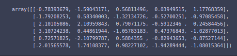
And first 5 rows of the resultant dataset are

X_train_pca[:6, :]

And the explained variance ratio via

pca1.explained_variance_ratio_

How to choose the number of dimensions in PCA

In practice, when you have good computational power, we normally use Grid Search to find the optimum number of hyperparameters, and we also use it to find the number of principal components, which give the best performance.

If we lack good computational power, we have to choose the number of principal components by a tradeoff between the performance of the classifier and the computational efficiency.

Supervised Data Compression via Linear Discriminant Analysis (LDA)

LDA or Linear Discriminant Analysis is one of the famous supervised data compressions. As the name supervised might have given you the idea, it takes into account the class labels that are absent in PCA. It is also a linear transformation technique, just like PCA.

LDA uses quite a similar approach to PCA, in the sense that we decompose the matrix into eigenvectors and eigenvalues, which then forms a lower-dimensional feature space. However, it uses a supervised approach, meaning that it takes into account the class labels.

Before applying LDA to our data, we assume that our data is normally distributed, the classes have identical covariance matrices, and the training examples are statistically independent of each other. It has been proved from some research papers that if one, or more, of these assumptions are violated slightly, LDA still works pretty well.

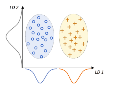
Source: Python Machine Learning Github Repo.

This graphic summarizes the concept of LDA for the 2-class problem, where circles are class 1 and + are class 2. A linear discriminant LD 1 (x-axis) would separate the 2 normally distributed classes well. Whereas the linear discriminant LD 2 captures a lot of variance in the dataset, it would fail as it would not be able to gather any class discrimination information.

In LDA, what we basically do is compute the within-class and between-class scatter matrices. Then, we compute the eigenvectors and corresponding eigenvalues for the scatter matrices, sort them in decreasing order, and select the top k eigenvectors that correspond to the k largest eigenvalues for constructing a d x k-dimensional transformation matrix W. We then project the examples in new feature subspace.

We can compute the within-class scatter matrix using the following formula:

where c is the total number of distinct classes, and Si is the individual scatter matrix of class i calculated via:

where mi is the mean vector that stores the mean feature value μm with respect to the example of class i.

Similarly, we can compute the between-class scatter matrix Sb:

Here, m is the overall mean that is computed, including examples from all c classes.

This whole work is not that difficult in Python and Numpy, and a lot of people have already done it. If you want to look at in detailed from-scratch implementation, have a look at this repo.

Let’s have a look at its implementation in sklearn in Python.

from sklearn.discriminant_analysis import LinearDiscriminantAnalysis as LDA
# we have already preprocessed the dataset in PCA, we will use the same dataset

LinearDiscriminantAnalysis is a class implemented in sklearn’s discriminant_analysis package. You can have a look at the documentation here.

The first step is to create an LDA object.

lda = LDA()
X_train_lda = lda.fit_transform(X_train_std, y_train)
X_test_lda = lda.transform(X_test_std)

An important thing to notice here is that in fit_transform function, we are passing the labels of the data set, and, as discussed earlier, it is a supervised algorithm.

Here we haven’t set n_components a parameter, so it will automatically decide to pick from the formula min(n_features, n_classes — 1). If we implicitly provide any value greater than this, it will give us an error. Check the documentation for more details.

We can check out the resultant shape via

X_train_lda.shape
>>> (124, 2)

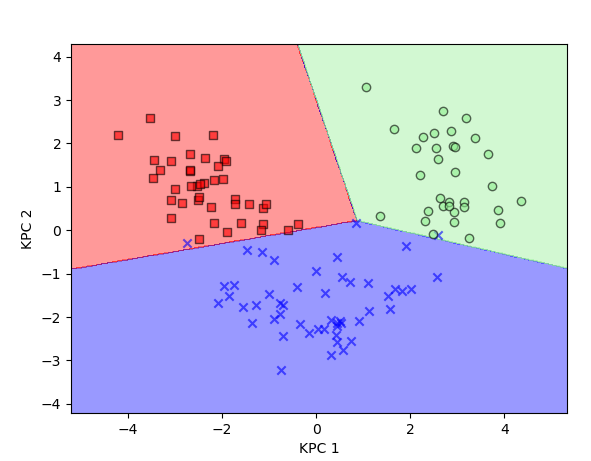
Since it is in 2 dimensions, we can easily plot all the classes. We will use the same code as above for plotting.

colors = ['r','b','g']
markers = ['s','x','o']
for l,c,m in zip(np.unique(y_train), colors, markers):
    plt.scatter(X_train_lda[y_train==l,0],
                X_train_lda[y_train==l,1],
                c=c, label=l, marker=m)
plt.title("Compressed Data")
plt.xlabel("LD 1")
plt.ylabel("LD 2")
plt.legend()
plt.tight_layout()
plt.show()

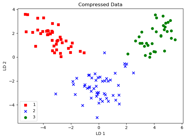
Now, as we have compressed the data, we can easily apply any machine learning algorithm to it. We can see that this data is easily linearly separable, so Logistic Regression would give us quite a good accuracy.

One thing we have to note in LDA via sklearn is that we can not provide n_components in probabilities as we can do in PCA. It must be an integer, and it must fulfill the condition min(n_features, n_classes — 1).

LDA vs PCA

One thought you might have encountered is that since LDA also keeps in mind the class labels as its supervised algorithm, the results in some cases show that PCA performs better than LDA, such as in tasks like image recognition when each class consists of a small number of examples (PCA Vrtsis LDA, A. M. Martinez, and A. C. Kak, IEEE Transactions on Pattern Analysis and Machine Intelligence, 23(2)L 228-233, 2001).

Kernel PCA

As discussed earlier, both PCA and LDA are linear dimensionality reduction techniques. Similarly, most machine learning algorithms make assumptions about the linear separability of the data to converge perfectly.

But the real-world is not always linear, and most of the time, you have to deal with nonlinear datasets. So, we can see that linear dimensionality reduction techniques might not be the best choice for these kinds of datasets.

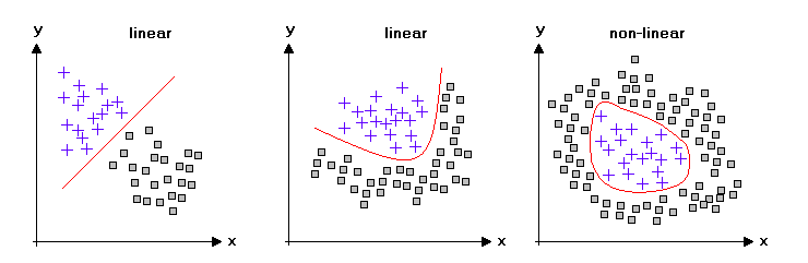
Image Credits: statistics4u.

Using KPCA, we can transform the data that is nonlinear to a linear subspace on which classifiers perform really well.

The main idea behind KPCA is that we have to perform a nonlinear mapping that transforms the data into a higher-dimensional space.

In other words, we transform our d-dimensional data to this higher k-dimensional space, and we define a nonlinear mapping function ϕ.

Think of ϕ as a function that maps the original d-dimensional dataset onto a larger, k-dimensional dataset via some nonlinear mappings.

In other words, we perform a nonlinear mapping to transform the dataset to a higher dimension where we use standard PCA to project the data back to a lower-dimension linearly separable space.

One downside of this approach is that it is very computationally expensive. To overcome this problem, we have to use the kernel trick, via which we can compute the similarity between two high-dimension feature vectors in the original feature space.

Now the mathematical details and intuition behind the kernel trick are difficult to explain in a written manner. I suggest you watch this video by the California Institute of Technology via which you can develop a good understanding of the mathematical intuition behind KPCA and kernel trick.

If you want to look at the implementation in Python and scipy, I recommend you to go through this repo where it is implemented step by step.

We will have a look at its implementation in sklearn in Python. What we are going to do is to convert a nonlinear 2-D dataset to a linear 2-D dataset. Remember, what KPCA will do is to map it to a higher dimension and then map it to a linearly separable lower dimension.

from sklearn.datasets import make_moons #non-linear dataset
from sklearn.decomposition import KernelPCA
import matplotlib.pyplot as plt
import numpy as np

Here we have imported important libraries and datasets.

X, y = make_moons(n_samples=100)
print(X.shape)

And we can see that our dataset has 100 rows and 2 columns. Let us see the number of classes and their values in our dataset.

print("Number of Unique Classes", len(np.unique(y)), "\nUnique Values are", np.unique(y))

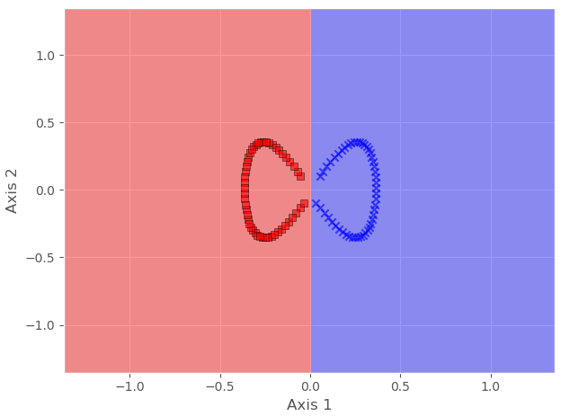
Since we have 2 classes, we can easily plot them.

#plotting the first class i.e y=0
plt.scatter(X[y==0,0], X[y==0,1],
            color = 'red', marker='^',
            alpha= 0.5)
#plotting the 2nd class i.e y=1
plt.scatter(X[y==1,0], X[y==1,1],
            color = 'blue', marker='o',
            alpha= 0.5)
#showing the plot
plt.xlabel("Axis 1")
plt.ylabel("Axis 2")
plt.tight_layout()
plt.show()

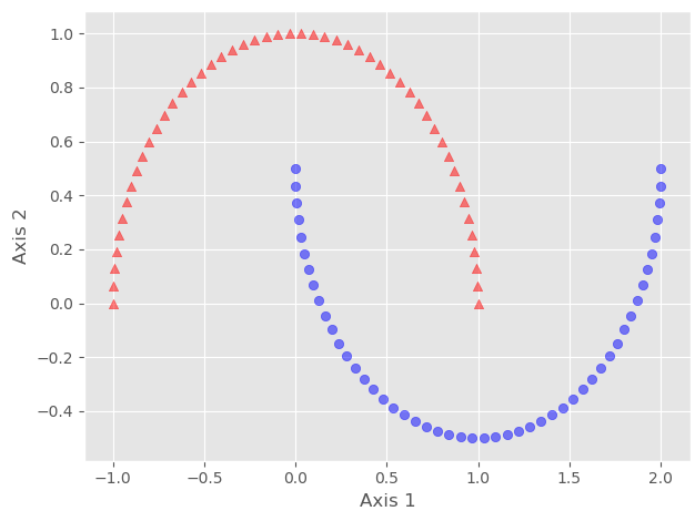
Here we can see that both classes are not linearly separable. We can confirm it by using any linear classifier.

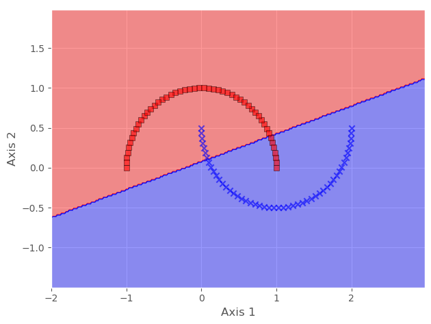
Hence, to make it linearly separable, we will cast it to a higher dimension, then map it back to a lower dimension, all using KPCA.

kpca = KernelPCA(n_components=2, kernel='rbf', gamma=15) #defining the KenrelPCA object

Here we have used the kernel='rbf' and gamma=15. There are different kernel functions that are to be used. Some of them are linear, poly, and rbf. Similarly, gamma is the kernel coefficient for the rbf, poly, and sigmoid kernels. There is a detailed answer on stats.StackExchange about which kernel to choose that you can read here.

Now we simply have to transform our data.

X_kpca = kpca.fit_transform(X) #transforming our dataset

Let us plot to check whether it is Linearly separable now or not.

plt.scatter(X_kpca[y==0,0], X_kpca[y==0,1],
            color = 'red', marker='^',
            alpha= 0.5)
plt.scatter(X_kpca[y==1,0], X_kpca[y==1,1],
            color = 'blue', marker='o',
            alpha= 0.5)
plt.xlabel("PCA 1")
plt.ylabel("PCA 2")
plt.tight_layout()
plt.show()

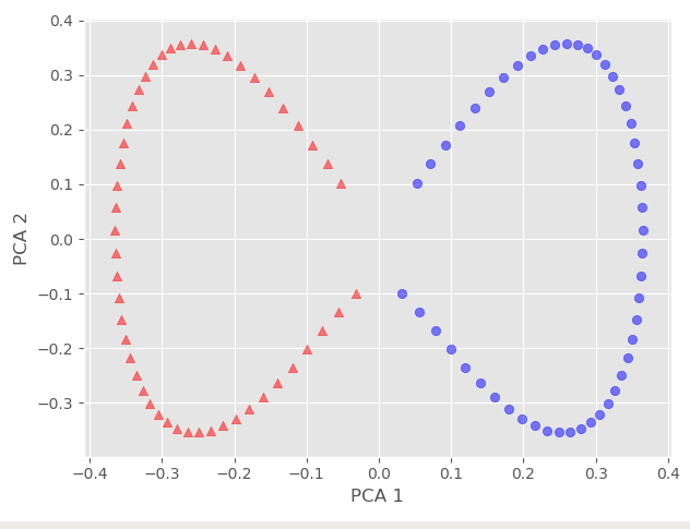
And we can see that our data is now linearly separable, and we can even confirm it via any linear classifier.

In this example, we have converted a nonlinear dataset into a linear dataset by using KPCA. In the coming example, we will decrease the dimensions of the wine dataset that we used previously in PCA and LDA.

kpca = KernelPCA(n_components=2)
X_train_kpca = kpca.fit_transform(X_train_std)
X_test_kpca = kpca.transform(X_test_std)

And this will transform our previous 13-dimensional data into 2 dimensional linearly separable data. We can now use any linear classifier to get good decision boundaries and good results.

Learning Outcomes

In this article, you learned the basics of 3 dimensionality reduction techniques in which 2 are linear, and 1 is nonlinear or uses the kernel trick. You have also learned their implementation in one of the most famous Python libraries, sklearn.